Yours is a classical problem of clock synchronization. You have a
software clock (your program's idea of the current time) which you want
to keep in sync with a reference hardware clock (the RTC). This is
typically achieved by using a phase-locked
loop, or PLL. It works
as follows:
- you measure the difference between your software clock's time and the
reference time
- you adjust your software clock based on this measurement.
This is essentially what you are already doing, except that you are
fixing your clock by stepping it abruptly, whereas a PLL would usually
slew the clock to get it in sync progressively.
Stepping the clock has some undesirable effects: it makes the time
discontinuous and, more annoyingly, it can make it non-monotonic. I
would thus recommend you try to slew your clock instead.
Here is the approach I would try if I were in your shoes. I am assuming
you are using an Arduino Uno, or a similar AVR-based board with a 16-bit
Timer 1:
- configure Timer 1 in mode 4: CTC mode with TOP = OCR1A
- set the prescaler to 64 and OCR1A = 12499 in order to get a period of
50 ms; TIMER1_COMPA_vect will be your data gathering interrupt
- configure your RTC to generate a 1 Hz output, and route this
signal to the input capture pin ICP1 (pin 8 on the Uno)
- run the PLL logic inside TIMER1_CAPT_vect.
Since the RTC's 1 Hz period is a multiple of the timer period, you
would expect the timer's input capture unit to always capture the same
value. The difference between two consecutive captured values is thus a
direct measure of your clock's drift in units of 4 ppm
(4 µs/s). The ISR would be basically along these lines:
ISR(TIMER1_CAPT_vect)
{
    static uint16_t last_capture;
    uint16_t this_capture = ICR1;
    int16_t drift = this_capture - last_capture;
    last_capture = this_capture;

    // Reduce the drift modulo 12500 into [-6250, +6250).
    if (drift >= 6250) drift -= 12500;
    if (drift < -6250) drift += 12500;

    tune_clock(drift);
}
where tune_clock() is your PLL algorithm responsible for slewing the
software clock.
Pay attention to the signedness of the variables. The subtraction of the
captured values should be done with unsigned numbers, then the result
should be made signed.
Edit: as suggested by James Waldby, I'll give here some suggestions
on the implementation of the PLL. It turns out it is not so simple:
measuring a clock drift is easy, predicting it is harder.
Let me restate the problem. You have a “good” clock: the RTC 1 Hz
signal, assumed to be perfect, but with a limited resolution of one
second. And you have a “bad” clock: Timer 1, which has a 4 µs resolution
but suffers from frequency inaccuracy, instability and sensitivity to
temperature and supply voltage. You want to combine
both clocks into a software clock which tracks the good clock yet has
the superior resolution of the bad clock.
I will use the following notations:
- t is the time from the reference clock (the RTC), assumed to be also
the physical time
- n = ⌊t⌋ is the integer part of t, which is also the time when we last
got an update from the RTC (a timer capture event)
- t′ is the time from the local clock (the Arduino timers)
- x = t′ − t is the local clock offset, measured by the ISR above at
integer values of t; the physical time is given by t = t′ − x
- y = dx/dt is the local clock drift rate; it's a dimensionless quantity
and typically less than 10−3 (i.e. less than 1 ms/s)
- xe(t) is the estimate, made by the software, of the offset x(t)
- ye(t) = dxe/dt is the estimate of the drift rate y(t)
- te = t′ − xe(te) is our software
clock: a self-consistent estimate of t
The simplest solution, which is equivalent to the one you have in your
question, is to assume x stays constant until it is updated. Thus
xe(t) = x(n)
te = t′ − x(n)
In other words, we are just correcting for the last known offset. The
problem is, as stated before, that this gives a discontinuous time
scale.
A better solution is to try to predict x(n+1), and linearly
interpolate between our previous and our current prediction, thus
building a continuous piecewise linear estimate of x:
xe(t) = xe(n) + (t−n)ye(n+½),
where ye(n+½) = xe(n+1) − xe(n)
From this, the estimated time can be solved for as:
te = n + (t′−xe(n)−n)/(1+ye(n+½))
≈ n + (t′−xe(n)−n)⋅(1−ye(n+½))
The factor 1/(1+ye(n+½)) ≈ (1−ye(n+½)) accounts
for the fact that the clock has drifted since the last update at t = n.
Now we are left with the problem of predicting x(n+1). There are
many possible approaches, and I will try to describe only a few.
Simple PLL
One simple approach is to simulate an analog PLL with a first order
low-pass filter. Here is the first illustration of the Wikipedia article
on phase-locked loop:

Some translation is needed between this analog picture and the digital
domain: The phase comparator takes the difference between the measured
offset x(n) and our previous prediction xe(n). The low pass
filter is implemented as an exponentially weighted moving average. The
output of the filter is our estimate of the drift rate: ye.
The VCO is the formula for estimating te, which has the
built-in drift rate −ye. This could be translated to C++
roughly along these lines:
struct {
    uint32_t n;  // time of last update
    float xe;    // estimate of offset at time n
    float ye;    // estimate of drift rate for t in [n ,n+1]
} clock;

const float tau = 60;  // low-pass filter time constant, in seconds
const float K = 1;     // DC gain of the filter
const float alpha = 1/(1+tau);

// Called by the ISR.
// y is (x[now] - x[1 second ago]) in units of 4 us.
void tune_clock(int16_t y)
{
    static float x;   // last known offset
    x += y * 4e-6;    // update known offset
    float xe = clock.xe + clock.ye;  // estimate of current offset

    // Update time.
    clock.n++;

    // Update our estimate of the drift rate.
    clock.ye += alpha*(K*(x-xe) - clock.ye);

    // Update or estimate of the offset.
    clock.xe = xe;
}

// Estimate the current time.
float time()
{
    float t_local = micros() * 1e-6;
    return clock.n + (t_local - clock.xe - clock.n) * (1 - clock.ye);
}
Note that the code above is only meant as a guide. A good implementation
should use fixed-point instead of floats and should also be
rollover-safe.
The time constant of the filter should be chosen large enough to smooth
out the jitter caused by the 4 µs resolution, yet short enough to
closely track the frequency variations of the local clock. Ideally, it
should be close to the Allan intercept of the x(n) time series.
This kind of PLL normally does a good job at tracking the reference
clock, but it has one drawback: it tends to carry a systematic offset.
Let's assume, for simplicity, that the drift rate is constant. Then it
can be easily seen that the steady state of the PLL carries an offset
error:
te − t = x − xe = y/K
where K is the DC gain of the filter. A large gain minimizes this error,
but it does so at the expense of stability. Too large a DC gain and the
PLL will spontaneously go into large oscillations.
I assume it should be possible to get rid of this systematic bias by
using more sophisticated filters, maybe something like a PID, but I
do not want to dive into the complexities of such filters.
Simple linear extrapolation
Another way of estimating x(n+1), which does not suffer from systematic
bias, is to linearly extrapolate from the two last known values:
xe(n+1) = 2 x(n) − x(n−1)
This means we assume that the drift rate is constant on this
short time scale. The problem with this method is that it tends to
amplify the fluctuations due to the jitter. Assuming for example an
(overoptimistic) drift rate of 2 ppm, the measured offset will
alternate between having zero and 4 µs increments. The
extrapolation will predict every zero increment to be followed by
another zero increment, and every 4 µs increment to be followed by
another 4 µs increment, and thus it will always be wrong. The time
evolution would look as follows:
t[s]    0   1   2   3   4   5   6   7   8   9  10
x[µs]   0   0   4   4   8   8  12  12  16  16  20
xₑ[µs]  0   0   0   8   4  12   8  16  12  20  16
Brown's linear exponential smoothing
Brown's method is one of many linear extrapolation methods
meant to smooth-out noise in the data. It is based on running twice
the same low-pass filter on the input data:
s1 = low_pass(x)   // first smoothing
s2 = low_pass(s1)  // second smoothing
If τ is the time constant of the filter, then s1 is an
average of data which has, on average the age τ, whereas s2
has the age 2τ. When can then, at time t, do a linear extrapolation by
running a straight line through the points (t−τ, s1) and
(t−2τ, s2). This gives the following algorithm for updating
the estimates of the offset and the drift rate:
static float s1, s2;      // x smoothed once and twice
s1 += alpha * (x - s1);   // update s1
s2 += alpha * (s1 - s2);  // update s2

// Update or estimate of the offset.
clock.xe = xe;

// Extrapolate to estimate next offset.
xe = s1 + (s1-s2)*(tau+1)/tau;

// Update our estimate of the drift rate.
clock.ye = xe - clock.xe;
Here again, the optimal time constant should be of the order of the
Allan intercept. Note that the limit τ → 0 gives the simple
extrapolation of the previous section.
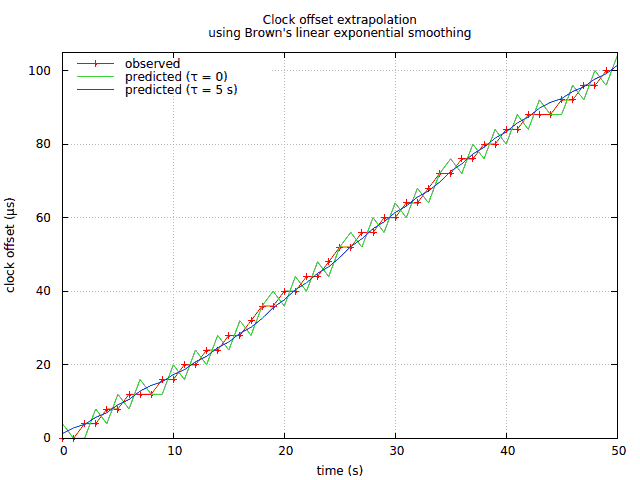
The figure below shows the performance of this algorithm on simulated
data. The simulated clock has a drift rate oscillating between 1.7 and
2.3 ppm, and its measured offset is rounded to the closest multiple of
4 µs. The line labeled “predicted (τ = 0)” is the simple
extrapolation of the previous section:

Here, the large jitter of the simple extrapolation method is quite
obvious. On this simulated data, Brown's method works well with a time
constant on the order of 5 s. The frequency of a real clock would
change much more slowly, and a longer time constant would work better.
Now, all this is probably too general for your particular use case. I
didn't know when I started this edit it would lead me so far... If you
can tolerate more than, say, 10 µs of jitter, then the simple
extrapolation should be good enough. And if you only need the time at
t′-periodic intervals, this may enable some optimizations.


getRTCTimeonly has 1sec resolution. So at the time of the request, it could be up to 999ms off. You could use the RTC to generate an interrupt every second, and connect that to an interrupt pin. Then in the pin-change interrupt check the difference between millis and a whole seconds counter. You can use that difference to get a calibrated millis. Not sure if this is the best solution.